fRFZP – IQClab

The second function allows removing all dynamics of a MIMO LTI system above a certain frequency $\omega$ . This function is useful, for example, to facilitate the implementation of a controller the has to be discretized, but has poles and\or zeros above the sampling frequency (which may very well happen when designing controllers in continuous time).

The operation proceeds by specifying $G_\mathrm{red}=fRFZP(G,\omega)$ , where $G$ is the original model and $\omega$ the cut-off frequency.

Example

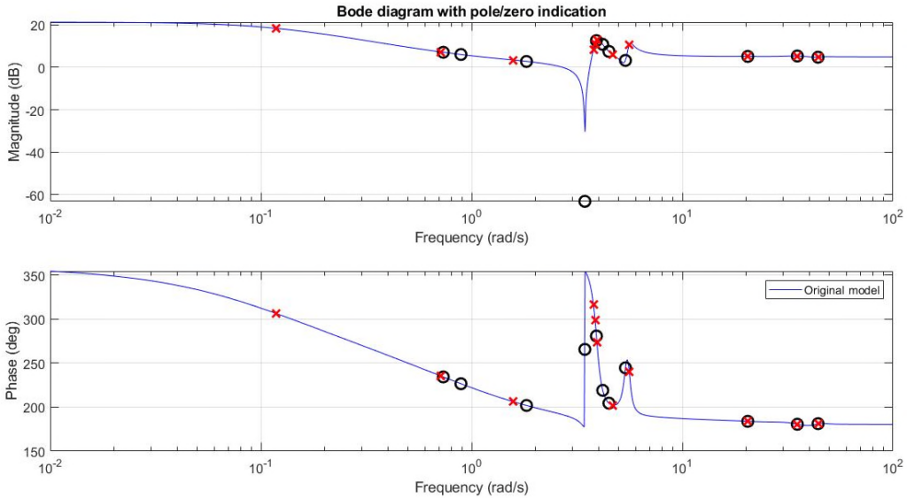
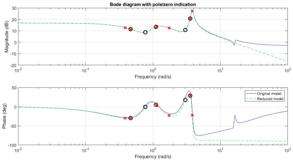
The following code generates a random LTI SISO state space model with 20 states. Subsequently the function fBodePZ (see details) plots the corresponding Bode diagram together with the poles and zeros of the model. This is shown in the figure below. The user is then asked to specify the cut-off frequency. With $\omega=7$ this yields the reduced order model shown in the second figure.

G = rss(20,1,1);
w = logspace(-2,2,1000);
fignr = 1;
fBodePZ(w,fignr,G,’b-‘,’Original model’);
Gred = fRFZP(G);
close(1)
fBodePZ(w,fignr,Gred,’g–‘,’Reduced model’,G,’b-‘,’Original model’);