LPV controller synthesis

IQClab also provides the option to perform LPV controller synthesis with full-block multipliers. This yields controllers that are gain-scheduled and depend on time varying parameters whose values are available via measurements or estimation algorithms.

Note: It is assumed that the user is acquainted with the LPV controller synthesis literature. The reader is referred to [7] and references therein for further information.

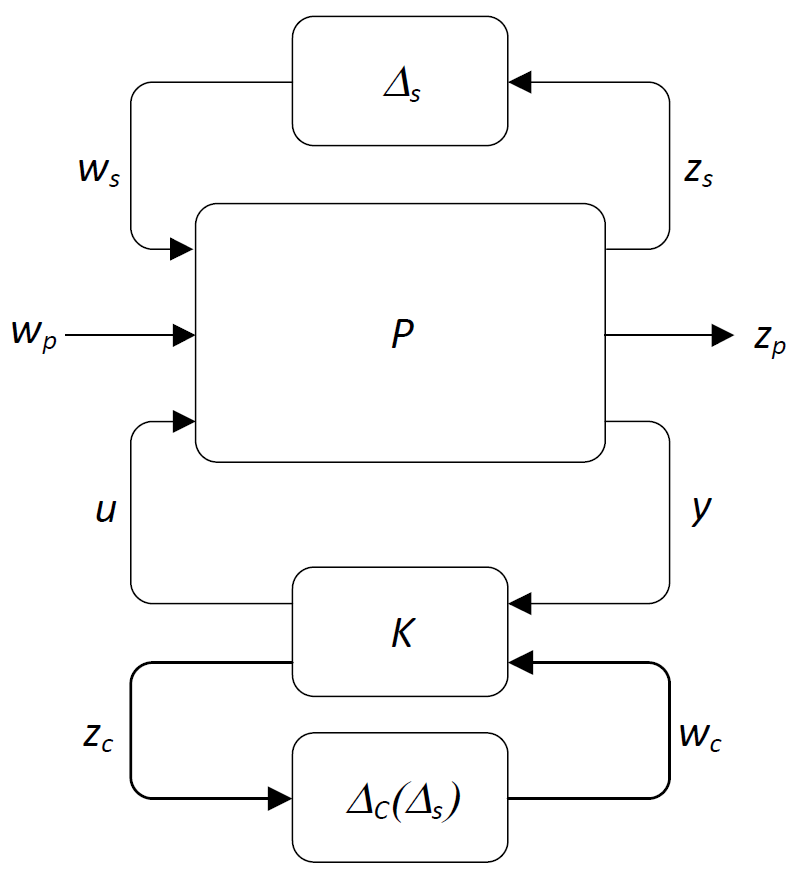
We consider the system interconnection shown in the following figure.

Here:

$P$ is the generalized plant (i.e., it is assumed that the disturbance and performance weights are already incorporated in the plant)
$\Delta_\mathrm{s}$ is the scheduling block, which depends on a time-varying parameter vector, which is further specified below
is the to-be-designed LPV controller, where
- $K$ is the LTI part
- $\Delta_\mathrm{c}(\Delta\mathrm{s})$ is the (nonlinear) scheduling function
the in- and output channels are denoted by
- $w_\mathrm{p}\rightarrow z_\mathrm{p}$ is the performance channel
- $w_\mathrm{s}\rightarrow z_\mathrm{s}$ is the plant scheduling function
- $w_\mathrm{c}\rightarrow z_\mathrm{c}$ is the controller scheduling channel
- $u\rightarrow y$ is the control channel

Some characteristics of the algorithm are:

The algorithms performs a synthesis with the aim to obtain a gain-scheduled controller,
$u=(k\star\Delta_\mathrm{c}(\Delta_\mathrm{s}))y,\ \ \ \ \Delta_\mathrm{c}(\Delta_\mathrm{s})=\left(\!\!\begin{array}{cc}0&\Delta_\mathrm{s}^T\\ \Delta_\mathrm{s}&0\end{array}\!\!\right)$
, which, for all $\Delta_\mathrm{s}\in\mathbf{\Delta}_\mathrm{s}$ , stabilizes the plant $\Delta_\mathrm{s}\star P$ and which renders the induced $L_2$ -gain on the channel $w_\mathrm{p}\rightarrow z_\mathrm{p}$ satisfied.
The block is a member of the uncertainty class ultv (see details here). This class is defined by LTV parametric uncertainties of the form
$\Delta_\mathrm{ultv}(\delta)=\sum_{i=1}^N\ldelta_iT_i=\delta_1T_1+\cdots+\delta_NT_N.$
Here
- $T_i$ , $i=\{1,\ldots,N\}$ are some fixed matrices $T_i\in\mathbb{R}^{n\times m}$ (having the same dimension as $\Delta_\mathrm{ultv}$ .
- $\delta:[0,\infty)\rightarrow\Lambda$ is a piecewise continuous time-varying parameter vector that takes its values from the compact polytope
  $\Lambda=\mathrm{co}\{\delta^1,\ldots,\delta^M\}=\left\{\sum_{a=1}^{M}b_a\delta^a: b_a\geq0,\ \sum_{a=1}^{M}b_a=1\right\}$
  with $\delta^a=(\delta_1^a,\ldots,\delta_N^a)$ , $a\in\{1,\ldots,M\}$ as generator points.
- $\Lambda$ is assumed to be star convex: $[0,1]\Lambda\subset\Lambda$ .
With the aim to trade-off computational complexity with performance, the algorithm allows to impose two different relaxation schemes:
- DG-scalings
- Convex Hull relaxation
The algorithm imposes the following induced $L_2$ norm constraint on the performance channel $w_\mathrm{p}\rightarrow z_\mathrm{p}$ :
$\int_0^{\infty}\left(\begin{array}{c}z_\mathrm{p}(t)\\w_\mathrm{p}(t)\end{array}\right)^T\left(\begin{array}{cc}\frac{1}{\gamma}I&0\\0&-\gamma I\end{array}\right)\left(\begin{array}{c}z_\mathrm{p}(t)\\w_\mathrm{p}(t)\end{array}\right)dt\geq0\ \ \forall t\geq0.$
Here $\gamma$ is the to-be-minimized induced $L_2$ -gain.

Usage:

$[K,\gamma]=fLPVsyn(P,\Delta,n_{out},n_{in})$
$[K,\gamma]=fLPVsyn(P,\Delta,n_{out},n_{in},options)$

If feasible, the algorithms returns:

The stabilizing controller $K$ with state space realization
$\left(\!\!\!\begin{array}{c}u\\z_\mathrm{c}\end{array}\!\!\!\right)\!=\!\left[\!\!\begin{array}{c|cc}A_\mathrm{c}&B_y&B_w\\ \hline C_u&D_{uy}&D_{uw}\\C_\mathrm{c}&D_{\mathrm{c}y}&D_{\mathrm{c}w}\end{array}\!\!\right]\!\!\!\left(\!\!\begin{array}{c}y\\w_\mathrm{c}\end{array}\!\!\!\right),$
where $y\rightarrow u$ is the control channel and $w_\mathrm{c}\rightarrow z_\mathrm{c}$ is the scheduling channel.
The (guaranteed) induced $L_2$ -gain on the performance channel $w_\mathrm{p}\rightarrow z_\mathrm{p}$ of the closed-loop system $(\Delta_\mathrm{s}\star P)\star(K\star\Delta_\mathrm{c}(\Delta_\mathrm{s}))$ .

The inputs should be provided as follows:

The LTI plant is assumed to admit the following state space description
$\left(\!\!\!\begin{array}{c}z_\mathrm{s}\\z_\mathrm{p}\\y\end{array}\!\!\!\right)\!=\!\left[\!\!\begin{array}{c|ccc}A&B_\mathrm{s}&B_\mathrm{p}&B_u\\ \hline C_\mathrm{s}&D_\mathrm{ss}&D_\mathrm{sp}&D_{\mathrm{s}u}\\C_\mathrm{p}&D_\mathrm{ps}&D_\mathrm{pp}&D_{\mathrm{p}u}\\C_y&D_{y\mathrm{s}}&D_{y\mathrm{p}}&D_{yu}\end{array}\!\!\right]\!\!\!\left(\!\!\begin{array}{c}w_\mathrm{s}\\w_\mathrm{p}\\u\end{array}\!\!\!\right),$
where
- $w_\mathrm{s}(\cdot)\in\mathbb{R}^{n_{w_\mathrm{s}}$ and $w_\mathrm{p}(\cdot)\in\mathbb{R}^{n_{w_\mathrm{p}}$ are the scheduling and disturbance inputs
- $z_\mathrm{s}(\cdot)\in\mathbb{R}^{n_{z_\mathrm{s}}$ and $z_\mathrm{p}(\cdot)\in\mathbb{R}^{n_{z_\mathrm{p}}$ are the scheduling and performance outputs
- $u(\cdot)\in\mathbb{R}^{n_u}$ is the control input
- $y(\cdot)\in\mathbb{R}^{n_y}$ is the measurement output
- $(A,B_u)$ is stabilizable and $(A,C_y)$ is detectable
The scheduling block $\Delta_\mathrm{s}(\delta)$ is an iqcdelta object, which must be compatible with the uncertainty class ultv (see details here).
The plant input and output dimension data and must be specified as follows:
- $n_\mathrm{in}=[n_{w_\mathrm{s}};n_{w_\mathrm{p}};n_{u}]$
- $n_\mathrm{out}=[n_{z_\mathrm{s}};n_{z_\mathrm{p}};n_{y}]$
The last input, options, is a structure with various options as summarized in the following table.

Options	Description
options.subopt	If chosen larger than 1, the algorithm computes a suboptimal solution $options.subopt\cdot\gamma$ , while minimizing the norms on the LMI variables $\\|X\\|<\gamma$ , $\\|Y\\|<\gamma$ , $\\|P_\mathrm{p}\\|<\gamma$ , $\\|P_\mathrm{d}\\|<\gamma$ . The default value is 1.05.
options.condnr	If chosen larger than 1, the algorithm computes a suboptimal solution $options.condnr\cdot\gamma$ , while improving the conditioning number of the coupling condition $\left(\begin{array}{cc}Y&\gamma I\\ \gamma I&X\end{array}\right)\succ0$ by maximizing $\gamma$ . The default value is 1.
options.Lyapext	With this option you can specify how the Lyapunov function matrix $X_e$ is constructed. The options are $options.Lyapext\in\{1,2,3,4,5\}$ . The default value is 5.
options.Multiplext	With this option you can specify how the extended multiplier matrix $P_\mathrm{e}$ is constructed. The options are $options.Multiplext\in\{1,2,3\}$ . The default value is 3.
options.constants	options.constants= $[c_1,c_2,c_3,c_4 <em>,c_5,c_6</em>]$ is a vector of (small) nonnegative constants, which perturb the LMIs as $LMI_i\prec-c_i$ , $i\in\{1,2,3,4,5,6\}$ . The constants are associated with the following LMI constraints – $c_1$ , $c_2$ perturb the coupling condition as $\left(\!\!\begin{array}{cc}Y&I\\I&X\end{array} \!\!\right)\!\succ\!\left( \!\!\begin{array}{cc}c_1I&0\\0&c_2I\end{array} \!\!\right)$ – $c_3$ perturbs the primal solvability condition as $LMI_\mathrm{primal}\prec-c_3I$ – $c_4$ perturbs the dual solvability condition as $LMI_\mathrm{dual}\succ c_4I$ – $c_5$ and $c_6$ perturb the multipliers as $\bullet^T \left(\!\!\begin{array}{cc}Q_\mathrm{p}& S_\mathrm{p}\\S_\mathrm{p}^T&R_\mathrm{p}\end{array} \!\! \right) \!\! \left( \!\! \begin{array}{c}I\\\Delta\end{array} \!\! \right)\!\succ\!c_5I,$ $\bullet^T\left(\!\!\begin{array}{cc}Q_\mathrm{d}& S_\mathrm{d}\\S_\mathrm{d}^T&R_\mathrm{d}\end{array}\!\!\right)\!\! \left(\!\!\begin{array}{c}-\Delta^T\\I\end{array}\!\!\right)\!\prec\!-c_6I,$ $Q_\mathrm{p}\!\succ \!c_5I\ \ R_\mathrm{d}\!\prec\!-c_6I$ The default value is $1e-9[1,1,1,1,1,1]$ .*
options.bounds	In case options.subopt>1, the algorithms miminizes the bounds $\\|X\\|<\gamma$ , $\\|Y\\| < \gamma$ , $\\|P_\mathrm{p}\\| < \gamma$ , $\\| P_\mathrm{d} \\| < \gamma$ . In case also the option options.bounds= $[b_1,b_2,b_3,b_4]$ is specified, one can scale the bounds on the LMI variables as $\\|X\\| < b_1\gamma$ , $\\|Y\\| < b_2\gamma$ , $\\|P_\mathrm{p}\\| < b_3\gamma$ , $\\| P_\mathrm{d} \\| < b_4\gamma$ , while minimizing $gamma$ . The matrices are empty by default.
options.gmax	This option specifies the maximum induced $L_2$ -gain bound on the performance channel $w_\mathrm{p}\rightarrow z_\mathrm{p}$ . The default value is 1000.
options.Parser	The option options.Parser specifies which parser is used: – options.Parser=’LMIlab’ – options.Parser=’Yalmip’ The default options is ‘LMIlab’.
options.Solver	The option options.Solver specifies which solver is used when considering Yalmip as parser. See https://yalmip.github.io/ for further info. The default solver is ‘mincx’.
options.FeasbRad	This option allows setting the feasibility radius of the optimization problem (see MATLAB → help → mincx for further details). The default value is 1e9.
options.Terminate	This option can be used to change the LMI solver options (see MATLAB → help → mincx for further details). The default value is 0.
options.RelAcc	This option can be used to change the LMI solver options (see MATLAB → help → mincx for further details). The default value is 1e-4.