
The file Demo_003.m is found in the IQClab’s folder demos. This demo performs a  – and IQC-robustness analysis for an uncertain plant that is affected by a delay uncertainty. Here it is possible to vary several inputs:
- xtrIQC
- Use the standard IQC-multiplier, or
- Use an extended one with an additional IQC-constraint
- Performance metric
- Induced
 -gain
-gain - Robust stability test
- Induced
The following uncertain plant was taken from [15].
% Define plant
s            = tf('s');
G            = ss(4/(s^2+0.1*s+1));
Gd           = ss(10/(s+0.1));
We           = 2/3*ss((s+3.674)^2/(s+0.03)^2);
Wu           = ss((s+10)/(s+1e4));
systemnames  = 'G Gd';
inputvar     = '[p;d;r;u]';
outputvar    = '[Gd;r-p-Gd;u;r-p-Gd]';
input_to_G   = '[u]';
input_to_Gd  = '[G+d]';
cleanupsysic = 'yes';
olic         = sysic;
wolic        = ssbal(blkdiag(1,We,Wu,1)*olic);
[K,CL,gamma] = hinfsyn(wolic(2:end,2:end),1,1);
M            = minreal(lft(wolic,K));
In this demo, we assume that the uncertainty block is defined by the  with
with ![\tau\in[0,\tau_\mathrm{max}]](https://usercontent.one/wp/www.iqclab.eu/wp-content/ql-cache/quicklatex.com-498b695ff3424883a98e85c5fbc9c8dd_l3.png?media=1702023987 "Rendered by QuickLaTeX.com") and
and  being the maximum time-delay.
The demo file Demo_003.m allows to run an IQC-analysis for various values of ![\alpha\in[0,0.05]](https://usercontent.one/wp/www.iqclab.eu/wp-content/ql-cache/quicklatex.com-25602d8fa2cd04f174b97078362cee64_l3.png?media=1702023987 "Rendered by QuickLaTeX.com") and within the file one can change the inputs mentioned above. For illustration purposes, the following 4 lines of code specify an IQC-analysis for the uncertain plant
and within the file one can change the inputs mentioned above. For illustration purposes, the following 4 lines of code specify an IQC-analysis for the uncertain plant  , with and
  , and the induced -gain as performance metric. In addition, the following parameters are considered:
- Length of the basis function: 3
- Extra IQC-constraint: ‘yes’
- Solution check: ‘on’
- Enforce strictness of the LMIs:

% M as above

% Define uncertainty block
de = iqcdelta('de','InputChannel',1,'OutputChannel',1, 'StaticDynamic','D','DelayType',1,'DelayTime',0.04);

% Assign IQC-multiplier to uncertainty block
de = iqcassign(de,'udel','Length',3 ,'AddIQC','yes');

% Define performance block
pe = iqcdelta('pe','ChannelClass','P','InputChannel',2, 'OutputChannel',2,'PerfMetric','L2');

% Perform IQC-analysis
prob = iqcanalysis(M,{de,pe},'SolChk','on','eps',1e-8);
If running the IQC analysis in Demo_003.m for
- xtrIQC: ‘No’ (Option 1.1)
- Induced -gain performance (Option 2.1)
you obtain the worst-case induced -gain for increasing values of ![\tau_\mathrm{max}\in[0,005]](https://usercontent.one/wp/www.iqclab.eu/wp-content/ql-cache/quicklatex.com-fd465d22a96f6358040e19b81d232326_l3.png?media=1702023987 "Rendered by QuickLaTeX.com") computed by the -tools (command: wcgain) and the IQC-tools for different lengths of the basis function. This yields the results shown in the following. As can be seen, the IQC-analysis produces worst-case induced -gains (i.e.,
computed by the -tools (command: wcgain) and the IQC-tools for different lengths of the basis function. This yields the results shown in the following. As can be seen, the IQC-analysis produces worst-case induced -gains (i.e.,  -norms in this example), which identical to the -analysis. In addition, dynamic IQC-multipliers seem not to have an advantage over static ones.
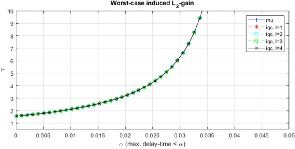 -gain for increasing maximum delay values
  and different lengths of the basis function (scenario: without extra IQC-constraint).
For comparison reasons, if running the IQC analysis in Demo_003.m for
- xtrIQC: ‘Yes’ (Option 1.2)
- Induced -gain performance (Option 2.1)
the IQC-analysis clearly offers an advantage over the -analysis at the cost of an extra computational load. This can be seen in the following figure.
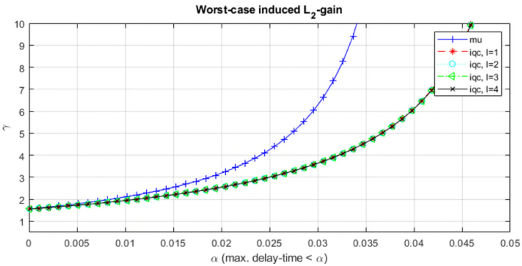 -gain for increasing maximum delay values and different lengths of the basis function (scenario: with extra IQC-constraint).