
The file Demo_002.m is found in IQClab’s folder demos. This demo performs a  – and IQC-robustness analysis for an uncertain plant that is affected by LTI dynamic uncertainties. Here it is possible to vary several inputs:
- The uncertainty block:
- One LTI dynamic
 uncertainty block, or
 - An LTI dynamic scalar uncertainty that is repeated twice
- One LTI dynamic
- Performance metric:
- Induced
 -gain
-gain  -norm
-norm- Robust stability test
- Induced
The uncertain system is given by  with the open-loop LTI plant
  , where
 ,
,  ,
,  ,
,  ,
,
while:
 for Option 3.1 and Option 3.3,
 for Option 3.2.
On the other hand, the uncertainty block is defined by:
 with
with  , for Option 1.1, or
 with
with  for Option 1.2.
The demo file Demo_002.m allows to run an IQC-analysis for various values of ![\alpha\in[0,0.5]](https://usercontent.one/wp/www.iqclab.eu/wp-content/ql-cache/quicklatex.com-cf9572b539b5d5923bb597eacc41be38_l3.png?media=1702023987 "Rendered by QuickLaTeX.com") and within the file one can change the inputs mentioned above. For illustration purposes, the following 5 lines of code specify an IQC-analysis for the uncertain plant
and within the file one can change the inputs mentioned above. For illustration purposes, the following 5 lines of code specify an IQC-analysis for the uncertain plant  , for
, for  and the -norm as performance metric. In addition, the following parameters are considered:
- Length of the basis function: 3
- Solution check: ‘on’
- Enforce strictness of the LMIs:

% Define uncertain plant
M = ss([-2,-3;1,1],[1,0,1;0,0,0],[1,0;0,0;1,0],[1,-2,0;1,-1,0;0,1,0]);

% Define uncertainty block
de = iqcdelta('de','InputChannel',[1;2], 'OutputChannel'[1;2],'StaticDynamic','D',
'NormBounds',0.2);

% Assign IQC-multiplier to uncertainty block
de = iqcassign(de,'ultid','Length',3);

% Define performance block
pe = iqcdelta('pe','ChannelClass','P','InputChannel',3, 'OutputChannel',3,'PerfMetric','H2');

% Perform IQC-analysis
prob = iqcanalysis(M,{de,pe},'SolChk','on','eps',1e-8);
To continue, if running the IQC-analysis in Demo_002.m for
- (Option 1.1)
- Induced -gain performance (Option 3.1)
you obtain as output the worst-case induced -gain for increasing values of computed by the -tools (command: wcgain) and the IQC-tools for different lengths of the basis function. This yields the results shown in the following figure. As can be seen, the IQC-analysis produces worst-case induced -gains (i.e.  -norms in this example), which are identical to the -analysis. In addition, note that for any length of the basis function, the same results are obtained. This means that static (i.e. non-dynamic) multipliers are sufficient in this analysis.
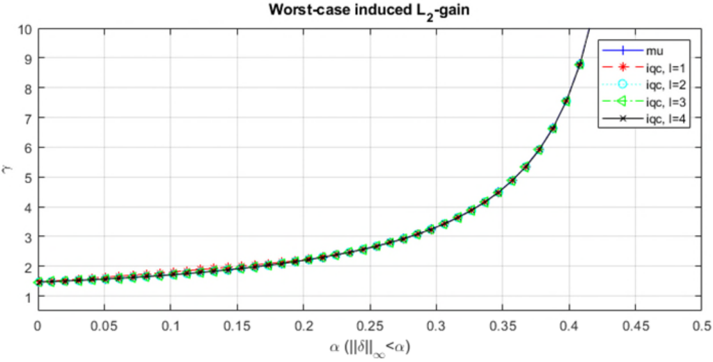 -gain for increasing values of
  and different lengths of the basis function